Volatility Measurement

In this post, we'll delve into various methods for measuring volatility, including close/close volatility, Parkinson volatility, Rogers/Satchell volatility, Garman/Klass volatility, and Yang/Zhang volatility. Our aim is to estimate the future realized volatility against the implied volatility provided by the options market to gain an edge.

Not only are we attempting to estimate a single future volatility point, but we're also aiming to estimate a range. However, it's not as straightforward as buying volatility because it's "cheap" or selling because it's "rich". Often, there's a reason behind these conditions, and we also need to utilize fundamental analysis. Are there any catalysts at play? Measuring volatility is an art form; there are over 100 volatility forecasting models, illustrating its complexity. There's no definitive right or wrong approach, only pros and cons to consider.

Volatility definition

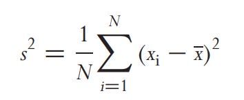
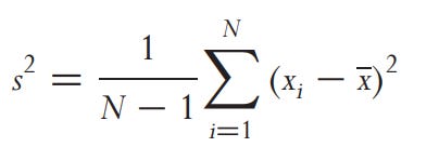
Volaitlity is the square root of the variance. Variance is

Where xi is the logarithmic return, x is the mean return, and N is the sample size. If we want to express the variance in annualized terms, we would need to multiply the variance by the annualization factor dictated by N. For daily data, this factor is 252. Additionally, we need to adjust the price for dividends and stock splits. For example, if we have a 3% price drop due to the stock going ex-dividend, it would be 48% annualized (Daily Volatility × square root(252)). You can achieve this normalization by using the adjustment factor dictated by this formula and multiplying it by the price before the ex-dividend date (backward adjustment).

The BSM model expects returns to be normally distributed, which is not the case, as we expect variance or volatility. Calculating the mean can be really noisy, especially in small sample sizes, so we set x (mean return) to 0 to remove noise.

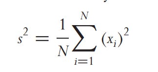
We need to convert it to population variance.

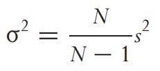
Always be aware of the N - 1 adjustment. Some people or institutions use sample variance (below), which is also used in VaR and has clear drawbacks when using x (mean return).

Annualized volatility is best calculated by multiplying by 20 or dividing by 20 (quick and dirty)

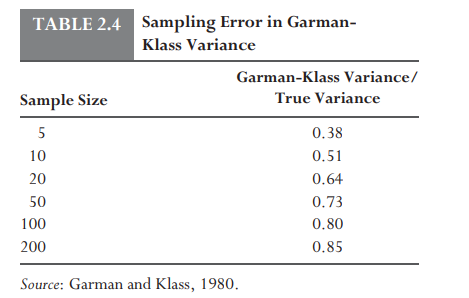
We discuss the efficiency (how quickly our estimated value converges to the true value) and bias (whether our method systematically estimates above or below the true value) of each estimator and also how each is perturbed by different aspects of real markets such as fat tails in returns, trends, and microstructure noise

Other Volatility Estimators

Parkinson

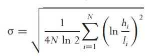
"h" is the high price and "l" the low price. This is normally how volatility is perceived by traders. It is five times more efficient than the close-to-close method but still underestimates volatility and is biased because prices may reach a high or low when we cannot observe them due to markets being open for only a certain time.

Garman and Klass

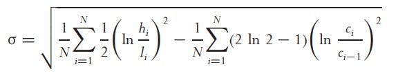
"c" represents the closing price. This method is up to 8 times as efficient as the close-to-close method but is also biased due to discrete sampling.

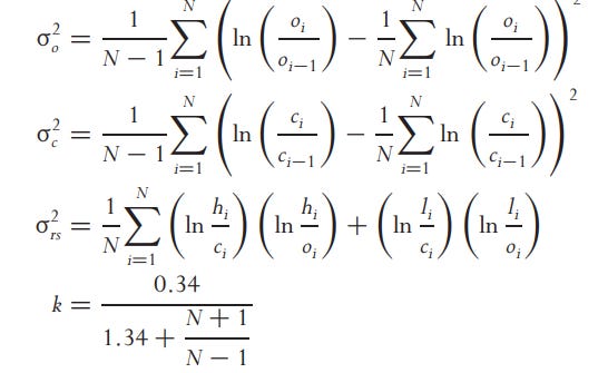
Rogers, Satchell, and Yoon

Rogers, Satchell, and Yoon outperform the others when drift is introduced, where "o" represents the closing price of the trading period.

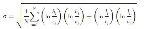
Yang and Zhang

Yang and Zhang can also account for jumps at the open by taking a weighted average of Rogers, Satchell, and Yoon.

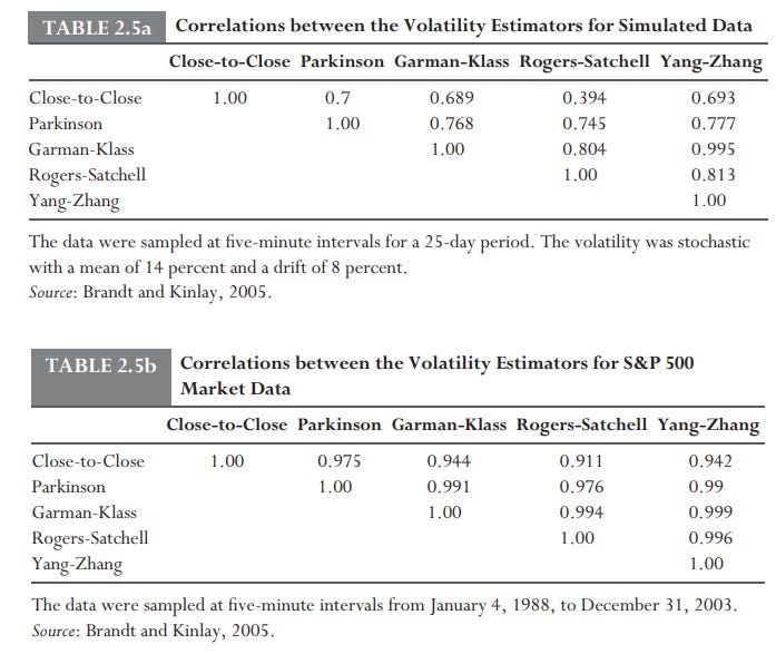
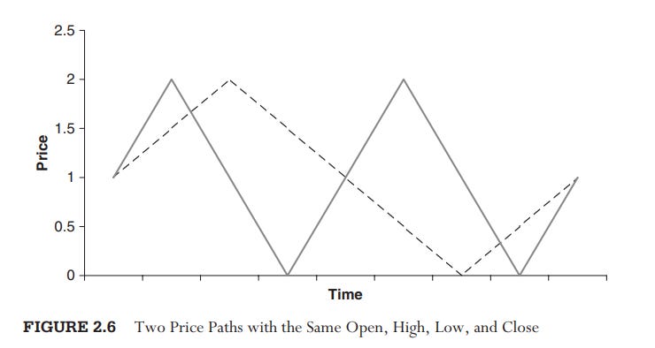
No one might say that there is a estimator that is the best, but this is not the case there are pros and cons. This table shows the correlation between the estimatiors

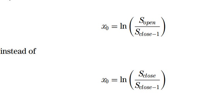
In essence, every one of the estimations uses OHLC data, which raises the question, “How far did the price move?”. Why not also ask, ‘‘How fast did the price move?’. Essentially, what you are doing is taking the open as 0% and then letting the price move the whole day while taking the log return from the open (delta) while dividing the price into a logarithmic price corridor which gets crossed at a certain time (t). This generates exit times

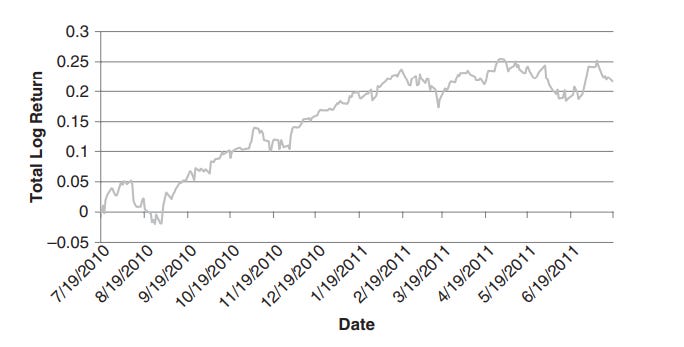
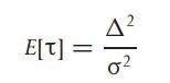
or

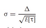
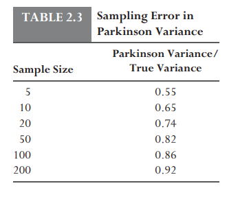
However, to avoid bias, we need to have a large sample size.

Here i will list the pros and cons of each estimator

Close-to-Close Estimator

Good Points

1. It has well-understood sampling properties.
2. It is easy to correct bias.
3. It is easy to convert to a form involving ‘‘typical daily moves.’’

Bad Points

1. It is an inefficient use of data and converges very slowly

Parkinson Estimator

Good Points

1. Using daily range seems sensible and provides completely separate information to using time-based samplings such as closing prices.

Bad Points

1. It is really only appropriate for measuring the volatility of a GBM process. In particular cannot handle trends and jumps.
2. It systematically underestimates volatility.

Garman-Klass Estimator

Good Points

1. It is up to eight times more efficient than close-to-close estimator.
2. It makes the best use of the commonly available price information.

Bad Points

1. It is even more biased than the Parkinson estimator.

Rogers-Satchell Estimator

Good Points

1. It allows for the presence of trends. VOLATILITY MEASUREMENT 28

Bad Points

1. It still cannot deal with jumps

Yang-Zhang Estimator

Good Points

1. It is specifically designed to have minimum estimation error.
2. It can handle both drift and jumps.
3. It is the most efficient in its use of available data.

Bad Points

1. The performance degrades to that of close-to-close estimator when process is dominated by jumps.

First Exit Time Estimator

Good Points

1. It uses fundamentally different information to traditional time-series methods.
2. It is a natural estimator for online use.
3. It converges relatively quickly.
4. It is not affected by the presence of noisy data or jumps.

Bad Points

1. It requires the use of high-frequency data.

Just remember, there is no best estimator; instead, we should consider what each indicator is telling us based on its pros and cons. For example, if Parkinson is 40% and close-to-close is 20%, we know that the volatility is being driven by big intraday ranges and closing prices are underrepresented in the process. This can help us determine when to hedge. For instance, ADRs will have predictable Parkinson/close ratios, as much new information is revealed when the stocks are not trading. You have to identify the environment.

As mentioned above, a larger sample size of your data helps us get more accurate volatility estimations. But not only a larger sample size, but also a higher frequency, such as one minute or less, is best. Using 15-minute prices, a 0.1 percent bid-ask spread can change our measurement by about 2 percent due to taking a noisy estimate of the true underlying price as our input. For options trading, starting with a 15 to 30-minute interval should work initially.

We have to account for several things. The seasonality on daily intervals does not matter that much; for example, on Monday and Friday, volatility is lower. What we have to account for are the overnight returns. To address this, we first calculate the open-to-close volatility and then the close-to-close volatility. After that, we have to weight both variances fairly. For stocks, 85% of the volatility happens in the trading hours; for indices, it's 90%; and for ADRs, it's 60% to 70%.

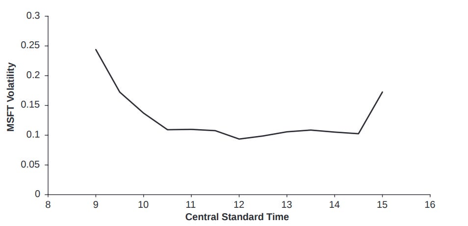
This is the average Parkinson volatility of 30-minute returns for the time period from April 23 to June 4, 2007. This pattern of volatility spiking at the open, slowing down midday, and then increasing again towards the end, has been observed in many instruments such as currencies, bonds, and equity indexes.

When we trade options, we are really interested in the average volatility over time (integrated volatility).

Some things to note:

1. Price can be instantaneously measured, while volatility cannot.
2. We need to estimate the average over time.
3. There are many volatility estimators, and when we have chosen one, there are several more parameters we have to choose.
4. Volatility measurement is an art.

As is said most of this is from this book which i encourage you to read

Thanks,

Finn