2024-03-21
Some known stylized facts:
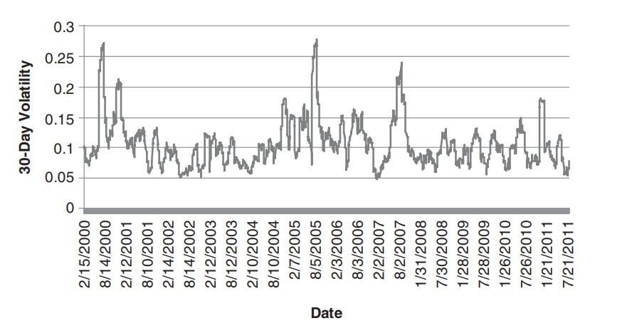
"Large changes tend to be followed by large changes, and small changes tend to be followed by small changes." - Mandelbrot. This statement reflects a principle often observed in various systems and phenomena, known as the "principle of amplification" or the "snowball effect." Essentially, it suggests that changes, whether large or small, can often lead to further changes of a similar magnitude. In many contexts, when a significant change occurs, it tends to have ripple effects or consequences that amplify its impact, leading to subsequent significant changes. This is known as Volatility Clusters. The graphic below illustrates this principle as well as the fact that volatility is not constant and changes in specific ways.
30-day close-to-close volatility of SPY from 2000 to 2011
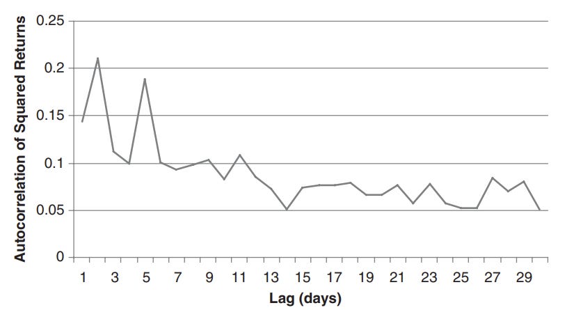
Both squared returns and absolute returns (proxies for one-day volatility) display significant autocorrelation. Below, you can see this autocorrelation for different lags, from which we can conclude that a good estimate of future volatility is whatever the current or yesterday's volatility is. However, this is only a rule of thumb because the underlying price does not have this property, which is the first reason that volatility is relatively predictable. The slow decay of the autocorrelation function is also referred to as ‘‘long memory.’’ Volatility clusters are observed in indices, stocks, commodities, and currencies.
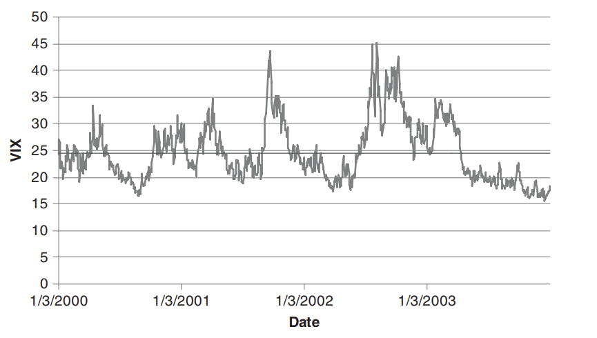
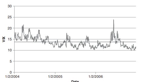
Volatility tends to revert to the mean, specifically short-term volatility tends to revert to the long-term mean. If the mean of daily volatility is higher than the mean of longer returns, we have a mean reversion. Volatility fluctuates, but over the long term, it isn't going anywhere. For example, the Volatility Index (VIX) has an annualized daily volatility of 0.96 (from 1990 to 2011), an annualized weekly volatility of 0.84, and an annualized monthly volatility of 0.59. However, it's important to note that it is often not possible to know the current value of the mean. If you look at the two graphics below, you can see how the mean is different for each period and always evolving. The interplay between clustering (positive autocorrelation) and mean reversion dominates the dynamics of volatility.
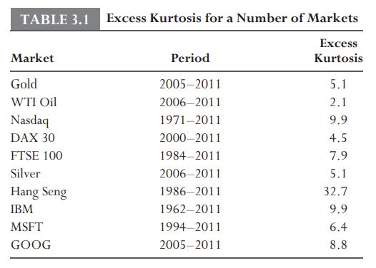
Returns in the financial world are not normally distributed; they mostly have fat tails (excess kurtosis) or are skewed.
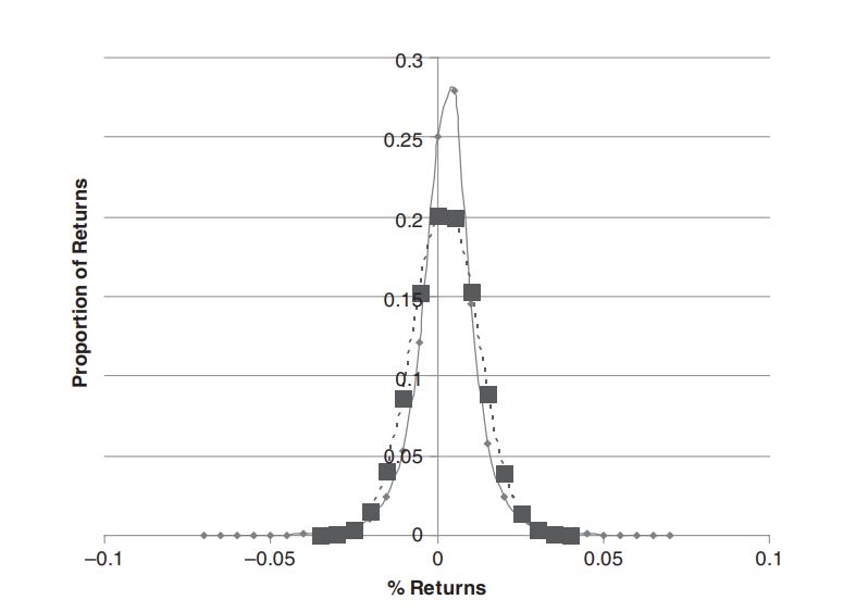
S&P 500 Daily Returns (Solid Line) and Those from a Normal Distribution (Dashed Line)
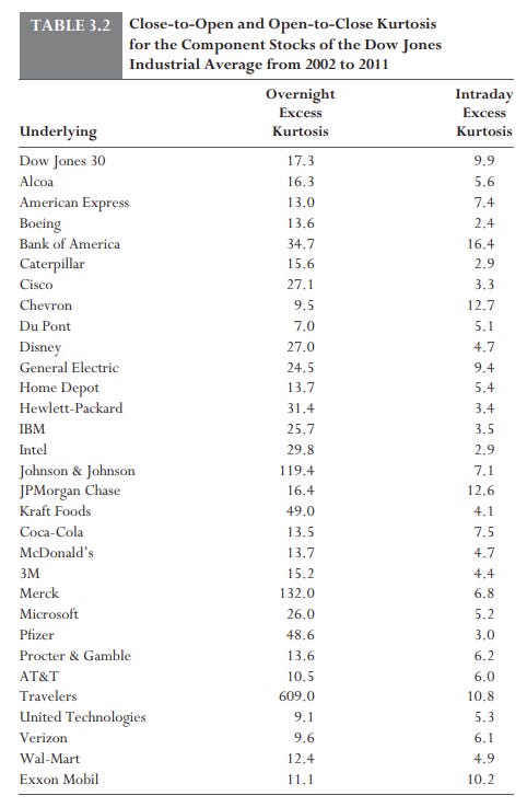
It's also interesting to note that the highest kurtosis occurs overnight, as most events or news happen when the market is not open, for example, earnings.
Volatility tends to increase when the underlying price declines. This is also known as the leverage effect. Assuming no debt is issued, a fall in the stock price causes the company’s financial leverage to increase, which increases its risk or leads to higher volatility. This is the theoretical explanation, but it does not always hold true in practice. This phenomenon mainly occurs in stock indices but is also true for single stocks, bonds, and many commodities—anything people invest in or which has a positive expected return. However, it doesn't apply to currencies. To observe the asymmetry in returns, you calculate the average size of positive returns and negative returns. Between 2000 and 2011, the average positive daily return for SPY was 0.008891, and the average negative return was -0.01007, 13% higher for the average negative return. Both fat tails and asymmetry are reflected in the structure of the implied volatility surface.
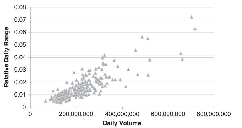
The SPY Daily Range Against the Daily Volume for 2011
Trading volume moves the underlying price, which causes volatility, but also increases volume for volatility-inducing investors to trade. You can also use volatility to avoid false signals.
The exact distribution is unimportant; it's more interesting that the distribution is heavily skewed to the left (with more occurrences of low volatility). Additionally, in bull markets, the average volatility is significantly lower than in bear markets.
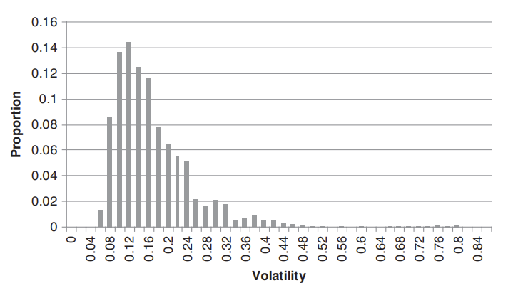
The Distribution of the 30-Day Volatility of the S&P 500 from 1990 to 2011
Common features
Most of this is from this book
Thanks,
Finn